PyTorch image classifier
Posted on Thu 26 April 2018 in Projects
from __future__ import print_function
import torch
Tensor oprations ref: http://pytorch.org/docs/stable/torch.html
# track computations with required_grad=True:
x = torch.ones(2, 2, requires_grad=True)
print(x)
y = x + 2
print(y)
# y was created as a result of an operation, so it has a grad_fn:
print(y.grad_fn)
# more operations on y:
z = y * y * 3
out = z.mean()
print(z, out)
# backprop:
out.backward()
print(x.grad)
Let's call the out Tensor "o". We have that
\begin{equation*}
o = \frac{1}{4}\sum_{i} z_i \;\; and \;\; z_i = 3(x_i + 2)^2 \;\; and \;\;\left.z_i\right|_{x_i = 1}=27.
\end{equation*}Therefore \begin{equation*} \frac{\partial o}{\partial x_i}=\frac{3}{2}(x_i+2), \;\; hence \;\; \left.\frac{\partial o}{\partial x_i}\right|_{x_i=1}=\frac{9}{2}=4.5 \end{equation*}
x = torch.rand(5,3)
print(x)
x = x.new_ones(5, 3, dtype=torch.double)
print(x)
print(x.size())
# (in place operations are post-fixed with _)
# standard numpy-like indexing works:
print(x[:,1])
Neural Nets in PyTorch
A typical training procedure for a neural network is as follows:
- Define the neural network that has some learnable parameters (or weights)
- Iterate over a dataset of inputs
- Process input through the network
- Compute the loss (how far is the output from being correct)
- Propagate gradients back into the network’s parameters
- Update the weights of the network, typically using a simple update rule:
weight = weight - learning_rate * gradient
Traning an image classifier:
1. Load and normalize CIFAR10 training and test datasets using torchvision (instead of boilerplate Pillow or OpenCV code)
import torchvision
import torchvision.transforms as transforms
transform = transforms.Compose(
[transforms.ToTensor(),
transforms.Normalize((0.5, 0.5, 0.5), (0.5, 0.5, 0.5))])
trainset = torchvision.datasets.CIFAR10(root='./pytorchdata', train=True,
download=True, transform=transform)
trainloader = torch.utils.data.DataLoader(trainset, batch_size=4,
shuffle=True, num_workers=2)
testset = torchvision.datasets.CIFAR10(root='./pytorchdata', train=False,
download=True, transform=transform)
testloader = torch.utils.data.DataLoader(testset, batch_size=4,
shuffle=False, num_workers=2)
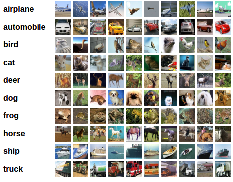
classes = ('plane', 'car', 'bird', 'cat',
'deer', 'dog', 'frog', 'horse', 'ship', 'truck')
show some of the training images, for fun:
import matplotlib.pyplot as plt
import numpy as np

def imshow(img):
    img = img / 2 + 0.5     # unnormalize
    npimg = img.numpy()
    plt.imshow(np.transpose(npimg, (1, 2, 0)))

# get some random training images
dataiter = iter(trainloader)
images, labels = dataiter.next()

# show images
imshow(torchvision.utils.make_grid(images))
# print labels
print(' '.join('%5s' % classes[labels[j]] for j in range(4)))

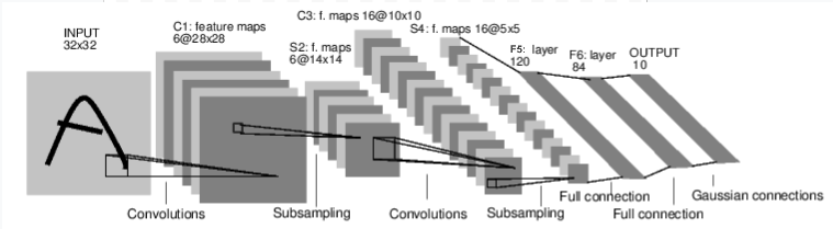
2. Define a Convolution Neural Net
It should take 3-channel images:
import torch.nn as nn
import torch.nn.functional as F

class Net(nn.Module):
    def __init__(self):
        super(Net, self).__init__()
        self.conv1 = nn.Conv2d(3, 6, 5)
        self.pool = nn.MaxPool2d(2, 2)
        self.conv2 = nn.Conv2d(6, 16, 5)
        self.fc1 = nn.Linear(16 * 5 * 5, 120)
        self.fc2 = nn.Linear(120, 84)
        self.fc3 = nn.Linear(84, 10)

    def forward(self, x):
        x = self.pool(F.relu(self.conv1(x)))
        x = self.pool(F.relu(self.conv2(x)))
        x = x.view(-1, 16 * 5 * 5)
        x = F.relu(self.fc1(x))
        x = F.relu(self.fc2(x))
        x = self.fc3(x)
        return x

net = Net()
3. Define a Loss function and optimizer
Use Classification Cross-Entropy loss and SGD with momentum:
import torch.optim as optim

criterion = nn.CrossEntropyLoss()
optimizer = optim.SGD(net.parameters(), lr=0.001, momentum=0.9)
4. Train
for epoch in range(2):  # loop over the dataset multiple times

    running_loss = 0.0
    for i, data in enumerate(trainloader, 0):
        # get the inputs
        inputs, labels = data

        # zero the parameter gradients
        optimizer.zero_grad()

        # forward + backward + optimize
        outputs = net(inputs)
        loss = criterion(outputs, labels)
        loss.backward()
        optimizer.step()

        # print statistics
        running_loss += loss.item()
        if i % 2000 == 1999:    # print every 2000 mini-batches
            print('[%d, %5d] loss: %.3f' %
                  (epoch + 1, i + 1, running_loss / 2000))
            running_loss = 0.0

print('Finished Training')
5. Test
predict the class label that the neural network outputs, and check it against the ground-truth. If the prediction is correct, we add the sample to the list of correct predictions.
First, display an image from the test set to get familiar.
dataiter = iter(testloader)
images, labels = dataiter.next()

# print images
imshow(torchvision.utils.make_grid(images))
print('GroundTruth: ', ' '.join('%5s' % classes[labels[j]] for j in range(4)))

# what does neural network think these examples are?
outputs = net(images)
print(outputs)
_, predicted = torch.max(outputs, 1)

print('Predicted: ', ' '.join('%5s' % classes[predicted[j]]
                              for j in range(4)))
correct = 0
total = 0
with torch.no_grad():
    for data in testloader:
        images, labels = data
        outputs = net(images)
        _, predicted = torch.max(outputs.data, 1)
        total += labels.size(0)
        correct += (predicted == labels).sum().item()

print('Accuracy of the network on the 10000 test images: %d %%' % (
    100 * correct / total))
That looks waaay better than chance, which is 10% accuracy (randomly picking a class out of 10 classes). Seems like the network learnt something.
Hmmm, what are the classes that performed well, and the classes that did not perform well:
class_correct = list(0. for i in range(10))
class_total = list(0. for i in range(10))
with torch.no_grad():
    for data in testloader:
        images, labels = data
        outputs = net(images)
        _, predicted = torch.max(outputs, 1)
        c = (predicted == labels).squeeze()
        for i in range(4):
            label = labels[i]
            class_correct[label] += c[i].item()
            class_total[label] += 1


for i in range(10):
    print('Accuracy of %5s : %2d %%' % (
        classes[i], 100 * class_correct[i] / class_total[i]))