DS Notebook 02
Posted on Wed 30 May 2018 in Projects
Using vectorization, ex. for efficient kNN calculation:
ufuncs in NumPy (vectorized expressions instead of loops)
import numpy as np
np.random.seed(0)

def compute_reciprocals(values):
    output = np.empty(len(values))
    for i in range(len(values)):
        output[i] = 1.0 / values[i]
    return output

values = np.random.randint(1, 100, size=1000000)
%timeit compute_reciprocals(values)
%timeit 1.0 / values
so, ufuncs much faster, since there is no type-checking. In a compiled language, that would've been taken care of already.
works with multi-dimensional arrays as well
x = np.arange(9).reshape((3,3))
x
x ** 2
The following table lists the arithmetic operators implemented in NumPy:
| Operator | Equivalent ufunc | Description |
|---|---|---|
+ |
np.add |
Addition (e.g., 1 + 1 = 2) |
- |
np.subtract |
Subtraction (e.g., 3 - 2 = 1) |
- |
np.negative |
Unary negation (e.g., -2) |
* |
np.multiply |
Multiplication (e.g., 2 * 3 = 6) |
/ |
np.divide |
Division (e.g., 3 / 2 = 1.5) |
// |
np.floor_divide |
Floor division (e.g., 3 // 2 = 1) |
** |
np.power |
Exponentiation (e.g., 2 ** 3 = 8) |
% |
np.mod |
Modulus/remainder (e.g., 9 % 4 = 1) |
Additionally there are Boolean/bitwise operators; we will explore these in Comparisons, Masks, and Boolean Logic.
Aggregations
| Function Name | NaN-safe Version | Description |
|---|---|---|
np.sum |
np.nansum |
Compute sum of elements |
np.prod |
np.nanprod |
Compute product of elements |
np.mean |
np.nanmean |
Compute mean of elements |
np.std |
np.nanstd |
Compute standard deviation |
np.var |
np.nanvar |
Compute variance |
np.min |
np.nanmin |
Find minimum value |
np.max |
np.nanmax |
Find maximum value |
np.argmin |
np.nanargmin |
Find index of minimum value |
np.argmax |
np.nanargmax |
Find index of maximum value |
np.median |
np.nanmedian |
Compute median of elements |
np.percentile |
np.nanpercentile |
Compute rank-based statistics of elements |
np.any |
N/A | Evaluate whether any elements are true |
np.all |
N/A | Evaluate whether all elements are true |
Computation on Arrays: Broadcasting
M = np.ones((3,3))
a = [1,2,3]
M + a
a = np.arange(3)
b = np.arange(3).reshape((3,1))

print(a)
print(b)
a + b
- Rule 1: If the two arrays differ in their number of dimensions, the shape of the one with fewer dimensions is padded with ones on its leading (left) side.
- Rule 2: If the shape of the two arrays does not match in any dimension, the array with shape equal to 1 in that dimension is stretched to match the other shape.
- Rule 3: If in any dimension the sizes disagree and neither is equal to 1, an error is raised.
X = np.random.random((10,3))
Xmean = X.mean(0)
Xmean
X_centered = X - Xmean
X_centered
X_centered.mean(0)
x = np.linspace(0, 5, 50)
y = np.linspace(0, 5, 50).reshape(50, 1)
# use broadcasting to compute z across the grid:
z = np.sin(x) ** 10 + np.cos(10 + y * x) * np.cos(x)
import matplotlib.pyplot as plt
plt.imshow(z, origin='lower', extent=[0, 5, 0, 5], cmap='viridis')
plt.colorbar();

Comparisons, Masks, Boolean Logic
Extract, modify, or otherwise manipulate values in an array based on some criterion. For example, count all values greater than a certain value, or remove all outliers above a threhold. In NumPy, Boolean masking is often most efficient.
x = np.array([1, 2, 3, 4, 5])
The result of ufunc comparison operators is always an array with a Boolean data type. <, >, <=, >=, !=, == are all available
x > 3
(2 * x) == (x ** 2)
rng = np.random.RandomState(0)
x = rng.randint(10, size=(3, 4))
x
x < 6
np.sum(x < 6)
^ False == 0 and True == 1 is used here
# how many values less than 6 in each row?
np.sum(x < 6, axis=1)
Can also use np.any(), np.all(), np.sum(), but these are different from built-in Python any(), all(), sum(), so be careful.
import pandas as pd
rainfall = pd.read_csv('Seattle2014.csv')['PRCP'].values
inches = rainfall / 254.0  # 1/10mm -> inches
inches.shape
np.sum((inches > 0.5) & (inches < 1))
| Operator | Equivalent ufunc | Operator | Equivalent ufunc | |
|---|---|---|---|---|
& |
np.bitwise_and |
| | np.bitwise_or |
|
^ |
np.bitwise_xor |
~ |
np.bitwise_not |
print("Number days without rain:      ", np.sum(inches == 0))
print("Number days with rain:         ", np.sum(inches != 0))
print("Days with more than 0.5 inches:", np.sum(inches > 0.5))
print("Rainy days with < 0.2 inches  :", np.sum((inches > 0) &
                                                (inches < 0.2)))
x
x < 5
# masking operation to select from array
x[x < 5]
# construct a mask of all rainy days
rainy = (inches > 0)

# construct a mask of all summer days (June 21st is the 172nd day)
days = np.arange(365)
summer = (days > 172) & (days < 262)

print("Median precip on rainy days in 2014 (inches):   ",
      np.median(inches[rainy]))
print("Median precip on summer days in 2014 (inches):  ",
      np.median(inches[summer]))
print("Maximum precip on summer days in 2014 (inches): ",
      np.max(inches[summer]))
print("Median precip on non-summer rainy days (inches):",
      np.median(inches[rainy & ~summer]))
One common point of confusion is the difference between the keywords and and or on one hand, and the operators & and | on the other hand.
When would you use one versus the other?
The difference is this: and and or gauge the truth or falsehood of entire object, while & and | refer to bits within each object.
When you use and or or, it's equivalent to asking Python to treat the object as a single Boolean entity.
In Python, all nonzero integers will evaluate as True.
bool(42), bool(0)
bool(42 and 0)
bool(42 or 0)
Notice that the corresponding bits of the binary representation are compared in order to yield the result. When you use & and | on integers, the expression operates on the bits of the element, applying the and or the or to the individual bits making up the number:
# bin() is binary representation of the number
bin(42)
bin(59)
bin(42 & 59)
A = np.array([1, 0, 1, 0, 1, 0], dtype=bool)
B = np.array([1, 1, 1, 0, 1, 1], dtype=bool)
A | B
A or B
x = np.arange(10)
(x > 4) & (x < 8)
(x > 4) and (x < 8)
So remember this: and and or perform a single Boolean evaluation on an entire object, while & and | perform multiple Boolean evaluations on the content (the individual bits or bytes) of an object.
For Boolean NumPy arrays, the latter is nearly always the desired operation.
Fancy Indexing
how to access and modify portions of arrays using:
- simple indices
arr[0] - slices
arr[:5] - Boolean masks
arr[arr > 0]
Fancy indexing is just passing an array of indices to access multiple array elements at once:
rand = np.random.RandomState(42)

x = rand.randint(100, size=10)
print(x)
[x[3], x[7], x[2]]
ind = [3, 7, 2]
x[ind]
ind = np.array([[3, 7],
                [2, 6]])
x[ind]
It is always important to remember with fancy indexing that the return value reflects the broadcasted shape of the indices, rather than the shape of the array being indexed.
x = np.zeros(10)
x[[0, 0]] = [4, 6]
x
i = [3, 3, 3]
x[i] += 1   # this *assignment* happens 3 times, but not the augmentation
x
to get the augmentation to happen multiple times, use at():
np.add.at(x, i, 1)
x
np.add.reduceat() is similarly useful..
Efficient manual histogram with searchsorted() and at()
np.random.seed(42)
x = np.random.randn(100)
x
bins = np.linspace(-5, 5, 20)
bins
counts = np.zeros_like(bins)
counts
i = np.searchsorted(bins, x)
i
np.add.at(counts, i, 1)
counts
bins
import matplotlib.pyplot as plt
import seaborn; seaborn.set()  # for plot styling
plt.plot(bins, counts, drawstyle='steps');

Sorting and Big-O
def selection_sort(x):
    for i in range(len(x)):
        swap = i + np.argmin(x[i:])
        (x[i], x[swap]) = (x[swap], x[i])
    return x
x = np.array([2, 1, 4, 3, 5])
selection_sort(x)
$N$ loops: for i in range(len(x)):
$N$ comparisons: np.argmin()
So, this sort function is slow, $\mathcal{O}[N^2]$
By default, NumPy's np.sort() function uses an $\mathcal{O}[N\log N]$ quicksort algorithm:
x = np.array([2, 1, 4, 3, 5])
np.sort(x)
x #x is unaffected
# sort in-place using .sort() method:
x.sort()
x
x = np.array([2, 1, 4, 3, 5])
i = np.argsort(x)
i
x[i]
rand = np.random.RandomState(42)
X = rand.randint(0, 10, (4, 6))
print(X)
np.sort(X, axis=0) # sort each column
np.sort(X, axis=1) # sort each row
x = np.array([7, 2, 3, 1, 6, 5, 4])
np.partition(x, 3)
np.partition(X, 2, axis=1)
The result is an array where the first two slots in each row contain the smallest values from that row, with the remaining values filling the remaining slots.
Finally, just as there is a np.argsort that computes indices of the sort, there is a np.argpartition that computes indices of the partition:
np.argpartition(X, 2)
Using np.newaxis to promote array to a higher dimension
a = np.arange(4)
a
a.shape
row_vec = a[np.newaxis, :]
row_vec.shape
col_vec = a[:, np.newaxis]
col_vec.shape
Example: kNN
X = rand.rand(200, 2)
plt.scatter(X[:, 0], X[:, 1], s=50);

Given $(x_1, y_1)$, $(x_2, y_2)$, ... $(x_n, y_n)$, first compute:
$x_1 - x_1$
$x_1 - x_2$
...
$x_n - x_n$
and
$y_1 - y_1$
$y_1 - y_2$
...
$y_1 - y_3$
differences = X[:, np.newaxis, :] - X[np.newaxis, :, :]
differences.shape
then square them.. $(x_1 - x_i)^2$ and $(y_1 - y_i)^2$:
sq_differences = differences ** 2
sq_differences.shape
then add the squared coordinate differences, so we have $(x_1 - x_i)^2 + (y_1 - y_i)^2$
dist_sq = sq_differences.sum(-1)
dist_sq.shape
dist_sq.diagonal()
nearest = np.argsort(dist_sq, axis=1)
print(nearest)
K = 3
nearest_partition = np.argpartition(dist_sq, K + 1, axis=1)
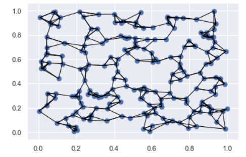
plt.scatter(X[:, 0], X[:, 1], s=50)

# draw lines from each point to its two nearest neighbors
K = 3

for i in range(X.shape[0]):
    for j in nearest_partition[i, :K+1]:
        # plot a line from X[i] to X[j]
        # use some zip magic to make it happen:
        plt.plot(*zip(X[j], X[i]), color='black', lw=1)

Structured Data
data = np.zeros(4, dtype={'names':('name', 'age', 'weight'),
                          'formats':('U10', 'i4', 'f8')})
print(data.dtype)
Here 'U10' translates to "Unicode string of maximum length 10," 'i4' translates to "4-byte (i.e., 32 bit) integer," and 'f8' translates to "8-byte (i.e., 64 bit) float."
name = ['Alice', 'Bob', 'Cathy', 'Doug']
age = [25, 45, 37, 19]
weight = [55.0, 85.5, 68.0, 61.5]
data['name'] = name
data['age'] = age
data['weight'] = weight
print(data)
data['name']
data[0]
data[-1][['name', 'age']]
data[data['age'] < 30]['name']
The shortened string format codes may seem confusing, but they are built on simple principles.
The first (optional) character is < or >, which means "little endian" or "big endian," respectively, and specifies the ordering convention for significant bits.
The next character specifies the type of data: characters, bytes, ints, floating points, and so on (see the table below).
The last character or characters represents the size of the object in bytes.
| Character | Description | Example |
|---|---|---|
'b' |
Byte | np.dtype('b') |
'i' |
Signed integer | np.dtype('i4') == np.int32 |
'u' |
Unsigned integer | np.dtype('u1') == np.uint8 |
'f' |
Floating point | np.dtype('f8') == np.int64 |
'c' |
Complex floating point | np.dtype('c16') == np.complex128 |
'S', 'a' |
String | np.dtype('S5') |
'U' |
Unicode string | np.dtype('U') == np.str_ |
'V' |
Raw data (void) | np.dtype('V') == np.void |